Differential Equations for a Railway Wheelset (Bogie)
Maple Workspace by B. Hassard, Uni-Ulm, Summer 1999

The equations are derived from the "more complex" model of

N. K. Cooperrider, "The Hunting Behavior of Conventional Railway Trucks",
Transactions of the ASME, Journal of Engineering for Industry 94 (1972) pp. 752-762,

which is given with fewer misprints, in

Ch. Kaas-Petersen, "Chaos in a Railway Bogie"
Acta Mechanica 61, 89-107 (1986)

Extensive simulations (but inaccurate points of Hopf bifurcation)are reported in

U. Galvanetto, L. Briseghella, S.R. Bishop "Optimal axle distance of a railway bogie",
International Journal of Bifurcation and Chaos Vol. 7, No. 3 (1997) 721-731

This workspace

(1) discusses misprints and inconsistencies in parameter values in the Kaas-Petersen paper,
(2) discusses differentiability properties of the system,
(3) derives explicit formulas for the 14-dimension system written in the form,
dy1dt = f1(y1,..,y14,v), .. dy14dt = f14(y1,..,y14,V)
(4) generates fortran code to evaluate the fi's and the Jacobian matrix
(5) calculates the Jacobian matrix at the origin for general V,

(6) calculates the value of v at which Hopf bifurcation occurs, solving alpha(v)=0,
for the 3 different values of b chosen by G.B.&B (1997)
where alpha(v) is the real part of the eigenvalue of largest real part for V=v,
in the 3 cases of short, medium, and long axle.

> reset(); Digits:=20; # Digits:=10 is standard..

>

(1a) K-P value for G, the stress modulus of steel, is too small by a factor of 100
When we calculate G pi a_e b_e from values given in the K-P paper,

> Gabvalues:={G=8.08E8, a_e=6.578E-3,b_e=3.934E-3};
Gpiabval[0]:=evalf(subs(Gabvalues,G*Pi*a_e*b_e));

(Since there is some uncertainty about the value for Gpiab, we index the possibilities
starting with index 0.)

Also in the K-P paper, a value is given for the product G*Pi*a_a*b_e:

> Gpiabval[1]:= 6.563E6;

so something is wrong.

A www.yahoo.de search for "shear modulus" found

http://www.mcelwee.net/German/html/properties_of_various_materials.html,

which lists G = 76 GPa for high carbon steel and G = 786 GPa for stainless steel.

Another search found a "units conversion" site

http://www.omnis.demon.co.uk/conversn/

giving
1 Pascal = 10 dyne/cm**2 = 10*10**(-5) Newtons/cm**2 = 1 Newton/meter**2,
so the shear modulus for carbon steel is 76 GPa = 76E9 Newtons/meter**2 = 7.6E10 N/meter**2.
The value 8.08E8 N/m**2 in the K-P paper (and repeated in Galvanetto, Briseghella, Bishop..)

is certainly too small.
So: assuming the product given in the K-P paper is correct, and the a_e, b-e are correct,
instead of G=8.08E8, K-P should probably have G=8.08E10.

> Gabvalues:={G=8.08E10, a_e=6.578E-3,b_e=3.934E-3};
Gpiabval[2]:=evalf(subs(Gabvalues,G*Pi*a_e*b_e));

This gives an exponent consistent with the value given for the product. but there is somewhat different
from the value 6.563E6 given by K-P.

>

(1b) Same symbols for size of contact ellipse and for other dimensions
The papers on this subject all use a and b, both for the dimensions of the contact ellipse, and also
a = 0.716 = half of the track gauge, and b = 1.074 = half of the axle distance. If we take these

values together in different combinations with the small incorrect value G,

> Gabvalues:={G=8.08E8, a=0.716, b_e=3.934E-3};
Gpiabval[3]:=evalf(subs(Gabvalues,G*Pi*a*b_e));
Gabvalues:={G=8.08E8, a_e=6.578E-3, b=1.074};
Gpiabval[4]:=evalf(subs(Gabvalues,G*Pi*a_e*b));
Gabvalues:={G=8.08E8, a=0.716, b=1.074};
Gpiabval[5]:=evalf(subs(Gabvalues,G*Pi*a*b));

Note: making Gpiab larger, causes the Hopf bifurcation to occur for smaller values of the parameter V.
For example, one could find a value for Gpiab, that would give rise to a Hopf bifurcation at v=65.40 meters/sec
with the 1.074 value for b. For the values of Gpiab listed above, the critical velocities for Hopf bifurcation are at

vvalue[1]:=68.644031211672181362; vvalue[3]:=68.199045949344306950; vvalue[4]:=65.776614047826677011;
vvalue[5]:=64.932693019575151203;

(1c) Discrepancy in the value of N
In the K-P paper, the values mu = 0.15 and mu N = 10E3 are both given. From these, we infer

> N = 10.0E3/0.15;

However, on p. 91 of the K-P paper, the following value is given:

> N = 66670;

It would be reasonable to assume either one of these values. Taking the value mu N = 10E3 is

making the first choice. However, one could also take

> mu*N = 0.15*66670;

The linearized system at the origin turns out to be independent of the value of mu N.
Therefore differences in this value cannot inflluence the location of the Hopf bifurcation.

>

(1d) Choices
There are various possible values for the products G pi a_e b_e and 2 for mu N, although since the Hopf
bifurcation point is independent of mu N, we shall just take mu N = 10000.

> ichoice:=1;
GpiabmuNvals := {Gpiab=Gpiabval[ichoice]} union {muN=10000};

>

(2) Continuity properties of the system.

The system fails to be smooth because of the square root in the definition of xi_R,which affects
continuity at the origin, and the piecewise definitions of F_R, and of F_T, which affect

continuity away from the origin.

Continuity at the origin
In a sufficiently small neighborhood of the origin, the only problem is the square root.
The dependence of the ksi_x's and the ksi_y's upon the q's is linear and therefore smooth.
So, the system will be as smooth in a neighborhood of the origin as the functions
F_x(ksi_x,ksi_y) and F_y(ksi_x,ksi_y), given by

> eq1:= F_x = (ksi_x/Psi)*F_R/ksi_R;
eq2:= F_y = (ksi_y/Phi)*F_R/ksi_R;

where (locally)

> eq3:= F_R = mu*N*(u - u**2/3 + u**3/27);
eq4:= u = (G*Pi*a_e*b_e/(mu*N))*ksi_R;
eq5:= ksi_R = sqrt((ksi_x/Psi)**2 + (ksi_y/Phi)**2);
subs(eq5,eq4);

Introducing scaled versions of ksi_x and ksi_y, define

> eq6:= eta_x = (G*Pi*a_e*b_e/(mu*N))*ksi_x/Psi;
eq7:= eta_y = (G*Pi*a_e*b_e/(mu*N))*ksi_y/Phi;
eq8:= eta_R = sqrt(eta_x**2+eta_y**2);
subs(eq6,eq7,eq8);

and since (G Pi a_e b_e/(mu N))>0, eta_R = u.

Replacing ksi_x, ksi_y and ksi_R in the definitions of F_x and F_y then gives

> ksisolns := solve({eq4,eq6,eq7},{ksi_x,ksi_y,ksi_R});
eq1a:= subs(ksisolns,eq1); eq2a:=subs(ksisolns,eq2);
eq1b:= subs(eq3,eq1a); eq2b:=subs(eq3,eq2a);

where u = eta_R = sqrt(eta_x**2+eta_y**2).

Let F_R1 denote the continuous extension (to u=0) of (1/(mu N))F_R(u)/u:

> F_R1 = 1 - u/3 + u**2/27;

Then, in terms of F_R1,

> eq1c:= F_x = mu*N*eta_x*F_R1(u);
eq2c:= F_y = mu*N*eta_y*F_R1(u);

Or, one may write

> eq1d:= F_x = mu*N*F_R2(eta_x,eta_y);
eq2d:= F_y = mu*N*F_R2(eta_y,eta_x);

where

> F_R2(eta1,eta2) = eta1*F_R1(sqrt(eta1**2+eta2**2));

Now consider the continuity properties of F_R2(eta1,eta2) near the origin.

The terms arising from 1 and u**2/27 in F_R1(u) are clearly smooth in eta1, eta1, so the
the continuity hinges on the term (-1/3)u.
So, consider eta1 sqrt(eta1**2+eta2**2) near the origin (eta2 sqrt(eta1**2+eta2**2) is similar).
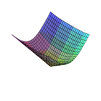
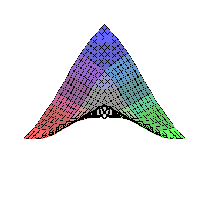
To investigate, we plot the first order partial derivatives:

> D1F:=diff(eta1*sqrt(eta1**2+eta2**2),eta1);
D2F:=diff(eta1*sqrt(eta1**2+eta2**2),eta2);
plot3d(D1F,eta1=-1..1,eta2=-1..1);
plot3d(D2F,eta1=-1..1,eta2=-1..1);
limit(limit(D1F,eta1=0),eta2=0);
limit(limit(D1F,eta2=0),eta1=0);
limit(limit(D2F,eta1=0),eta2=0);
limit(limit(D2F,eta2=0),eta1=0);

It is fairly clear that the first order partial derivatives of these functions are all continuous at the origin,
but that there are second order partial derivatives that are not.
Since eta_x and eta_y are linear homogenous in the variables y1..y14, it follows that the functions f1.. f14

in the sytem of DE's, are C1, but not C2, at the origin provided the function F_R(u)/ksi_R appearing in

the definitions, is replaced by its continuous extension.

>

(2b) Continuity away from the origin
The functions f1..f14 are smooth away from the origin, except on hypersurfaces corresponding to the
breakpoint u=3 in the piecewise defined function F_R, (F_R(u) is C2 but not C3 at u=3),
and the breakpoints u = delta and -delta in the function F_T. F_T is: smooth, except
1. at the origin where it is C1,
2. at points satisfying eta_Rf = 3 and eta_Rr=3, where it is C2,
3. on hyperplanes y1=+-delta and y3=+-delta, where it is C0

If integrating the system with a standard integrator, since the only terms involving F_T are F_T(y1) and F_T(y2)

one should stop the integration on crossing y1=+-delta, y3=+-delta, repeat the step to hit the point closely,
and then restart the integration. Otherwise, one can expect an O(h) or perhaps O(h**2) truncation error when
crossing over these points. The breakpoint for F_R poses a less serious problem, especially if a low order integrator

is used.

>

(3) Formulas for the functions f1..f14

>

> PsiPhivalues:={Psi=0.54219,Phi=0.60252};

It is simplest to express all 4 of the terms f_xf, f_yf, f_xr, f_yr in terms of a single nonlinear function.
Since Maple works better with Heaviside functions than with "if" conditions,

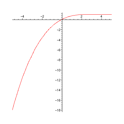
> FR0:=proc(u) (u-u^2/3+u^3/27)*Heaviside(3-u)+Heaviside(u-3)
end; # as in K-P paper

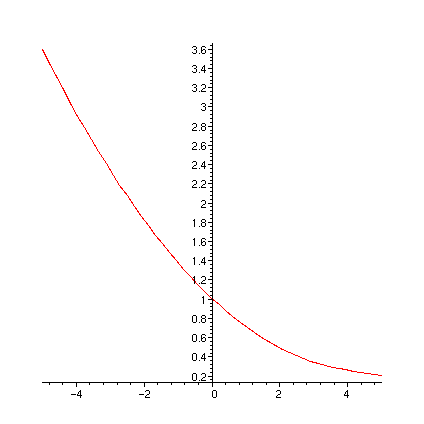
FR1:=proc(u) # used here (FR0(u)/u)
(1 - u/3 + u^2/27)*Heaviside(3-u)+(1/u)*Heaviside(u-3)
end;

FR1a:=proc(u) # same as FR1,
# but it generates better fortran code than FR1
# Maple can differentiate FR1, but not FR1a
if u<3 then (1 - u/3 + u^2/27) else 1/u fi end;
dFR1adu:= proc(u) # derivative of FR1a,
# for fortran code generation
if u<3 then -1/3 + 2*u/27 else (-1/u**2) fi end;

print(` FR0`); plot(FR0,-5..5);
print(` FR1`); plot(FR1,-5..5);
print(` FR1a`); plot(FR1a,-5..5);
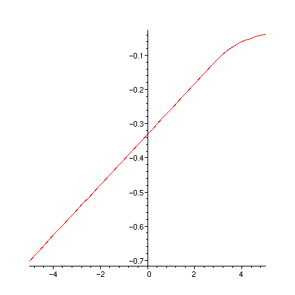
print(` diff(FR1(u),u)`); plot(diff(FR1(u),u),u=-5..5);
print(` dFR1adu`); plot(dFR1adu,-5..5);

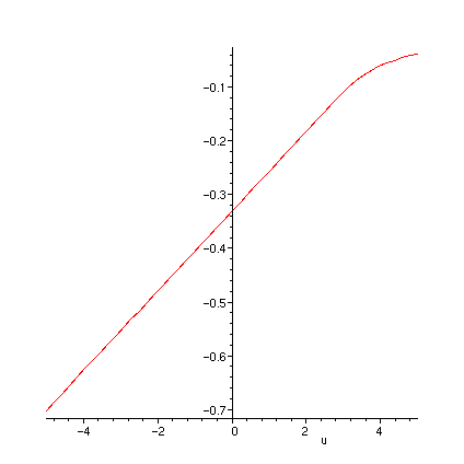
> FR2:=proc(eta1,eta2) eta1*FR1(sqrt(eta1^2+eta2^2)) end;

# the following are forms of FR2 and derivatives, for fortran code generation
FR2a:=proc(eta1,eta2) eta1*FR1(sqrt(eta1^2+eta2^2)) end;
D1FR2a:=proc(eta1,eta2)
if eta1=0 and eta2=0 then 1 else
FR1(sqrt(eta1**2+eta2**2))+
eta1*dFR1adu(sqrt(eta1**2+eta2**2))*
(1/2)*(1/sqrt(eta1**2+eta2**2))*2*eta1 fi end;
D2FR2a:=proc(eta1,eta2)
if eta1=0 and eta2=0 then 0 else
eta1*dFR1adu(sqrt(eta1**2+eta2**2))*
(1/2)*(1/sqrt(eta1**2+eta2**2))*2*eta2 fi end;


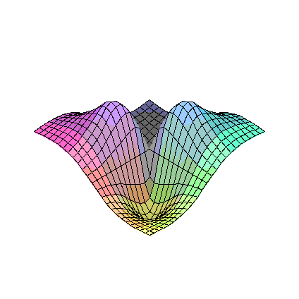
plot3d(FR2,-5..5,-5..5);

plot3d(diff(FR2(eta1,eta2),eta1),eta1=-5..5,eta2=-5..5);
limit(limit(diff(FR2(eta1,eta2),eta1),eta1=0),eta2=0);
plot3d(D1FR2a,-5..5,-5..5);
plot3d(diff(FR2(eta1,eta2),eta2),eta1=-5..5,eta2=-5..5);
limit(limit(diff(FR2(eta1,eta2),eta2),eta1=0),eta2=0);
plot3d(D2FR2a,-5..5,-5..5);

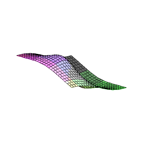
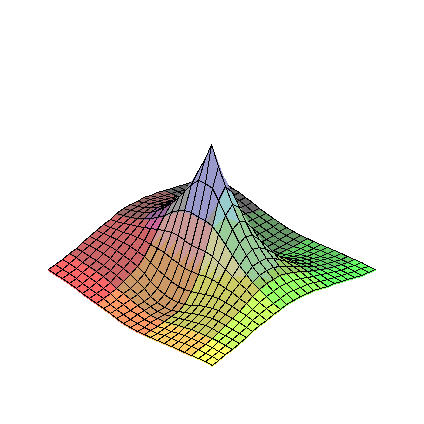
> k0deltavalues := {k0=14.6E6,delta=0.0091};

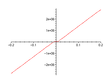
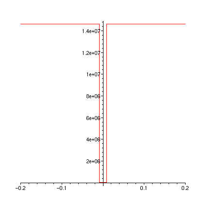
> FT:=proc(u)
subs(k0deltavalues,
k0*(u+delta)*Heaviside(-delta-u)+ k0*(u-delta)*Heaviside(u-delta));
end;
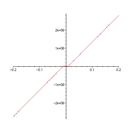
FTa:=proc(u)
local k0v,deltav;
# same as FT but translates better into fortran
k0v := subs(k0deltavalues,k0);
deltav := subs(k0deltavalues,delta);
if u<-deltav then k0v*(u+deltav)
elif u>deltav then k0v*(u-deltav)
else 0 fi; end;
dFTadu:=proc(u)
local k0v,deltav;
# derivative of FT, for translation into fortran
k0v := subs(k0deltavalues,k0);
deltav := subs(k0deltavalues,delta);
if u<-deltav then k0v
elif u>deltav then k0v
else 0.0 fi; end;

> plot(FT,-0.2..0.2);
plot(FTa,-0.2..0.2);
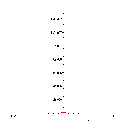
plot(diff(FT(u),u),u=-0.2..0.2);
plot(dFTadu,-0.2..0.2);

> bogievalues:={momega=1022,mf=2918,
Iomegay=678,Ify=6780,Ifr=6780,
a=0.716,b=1.074,
d1=0.620,d2=0.680,
h1=0.0762,h2=0.6584}:
lamr0values:={lambda=0.05,r0=0.4572}:
kDvalues:={k1=1.823E6,k2=3.646E6,k3=3.646E6,
k4=0.1823E6,k5=0.3333E6,k6=2.710E6,
D_1=20.0E3,D_2=29.2E3}:
paramvalues:=bogievalues union lamr0values union kDvalues;

>

The Ch. K-P paper uses ksi_xf, etc, but the equations have a slightly simpler formulation (using fewer procedures)
if instead, the ksi_xf etc. quantities are scaled into the following eta_xf etc. quantities..

> etaxf := (Gpiab/muN)*(dq1dt/V-q2)/Psi;
etayf := (Gpiab/muN)*(a*dq2dt/V+lambda*q1/r0)/Phi;
etarf := sqrt(etaxf^2+etayf^2);
etaxr := (Gpiab/muN)*(dq3dt/V-q4)/Psi;
etayr := (Gpiab/muN)*(a*dq4dt/V+lambda*q3/r0)/Phi;
etarr := sqrt(etaxr^2+etayr^2);
etaset := {eta_xf=etaxf,eta_yf=etayf,eta_xr=etaxr,eta_yr=etayr,
eta_rf=etarf,eta_rr=etarr};

Prepare substitutions for q's and derivatives, in terms of y's and derivatives

> qyset := {}:
for i from 1 to 7 do
qyset := qyset union {q.i = y.i} union {dq.i.dt=y.(i+7)}
union {d2q.i.dt2 = dy.(i+7).dt}:
od:
qyset;

In debugging this workspace, the equations were evaluated at the following point for comparision
of numerical values with output from the fortran code FCN for the bogie, due to C. Franke, provided by R. Seydel

> point1:={y1=1,y2=0,y3=1,y4=0,y5=0,y6=0,y7=0,y8=0,y9=0,y10=0,
y11=0,y12=0,y13=0,y14=0};

Prepare substitutions for the symbolic f_xf, f_yf,.. in terms of symbolic F_R2, eta_xf,..

Test by generating numeric values for f_xf,.. at point1

> fetaset:={f_xf=muN*F_R2(eta_xf,eta_yf),
f_yf=muN*F_R2(eta_yf,eta_xf),
f_xr=muN*F_R2(eta_xr,eta_yr),
f_yr=muN*F_R2(eta_yr,eta_xr)};
etasetv:=subs(GpiabmuNvals,etaset);
subs(F_R2=FR2,subs(PsiPhivalues,subs(GpiabmuNvals,subs(point1,subs(V=60,subs(paramvalues,subs(qyset,subs(etasetv,fetaset))))))));evalf(%);

The 2nd order differential equations from the K-P paper, in purely symbolic form (none
of the symbols involved, have values)

> qde1 := momega*d2q1dt2 + A1 + 2*f_xf + F_T(q1) = 0;
qde2 := Iomegay*d2q2dt2 + A3 + 2*a*f_yf = 0;
qde3 := momega*d2q3dt2 + A2 + 2*f_xr + F_T(q3) = 0;
qde4 := Iomegay*d2q4dt2 + A4 + 2*a*f_yr = 0;
qde5:= mf*d2q5dt2 - A1 - A2 + A5 = 0;
qde6 := Ify*d2q6dt2 - b*A1 + b*A2 - A3 -A4 + A6 = 0;
qde7 := Ifr*d2q7dt2 - h1*A1 - h1*A2 - h2*A5 + A7 = 0;

Substitute more legible symbols to display the set of equations in a form easily compared to the paper.
(The set of equations qde1 .. qde7 is not changed)

> legibleset:={}: for i from 1 to 7 do
legibleset:=legibleset union {q.i=q[i],dq.i.dt=diff(q[i](t),t),
d2q.i.dt2=diff(q[i](t),t$2),A.i=A[i]} od:
legibleset:=legibleset union
{momega=m[omega],Iomegay=I[omega*y],mf=m[f],
Ify=I[f*y],Ifr=I[f*r],h1=h[1],h2=h[2],
f_xf=f[xf],f_yf=f[yf],f_xr=f[xr],f_yr=f[yr],F_T=F[T]};
for i from 1 to 7 do
subs(legibleset,qde.i) od;

Form (first order) differential equations yde1, .. yde14 for y1 .. y14

> for i from 1 to 7 do yde.i := dy.i.dt=y.(i+7) od;
for i from 1 to 7 do yde.(i+7) := subs(qyset,qde.i) od;

Solve for the functions f1,..,f14 of the differential equations dy1dt = f1, .. dy14dt=f14

> for i from 1 to 14 do f.i := solve(yde.i,dy.i.dt); od;

In the differential equations, quantities A1,..,A7 appear. First prepare a set of definitions for
A1..A7 in terms of the q's., as in the K-P paper, then replace the q's and derivatives by y's
to obtain a set of definitions for A1..A7 in terms of the y's

> Aqset := {A1=2*k1*(q1-q5-b*q6-h1*q7),
A2=2*k1*(q3-q5+b*q6-h1*q7),
A3=2*k2*d1^2*(q2-q6),
A4=2*k2*d1^2*(q4-q6),
A5=2*D_2*(dq5dt-h2*dq7dt)+2*k4*(q5-h2*q7),
A6=k6*q6,
A7=2*D_1*d2^2*dq7dt+2*k5*d2^2*q7+4*k3*d1^2*q7};
Ayset := subs(qyset,Aqset);

Modify f1..f14 by replacing the symbols A1..A7 by their definitions in terms of the y's

> for i from 1 to 14 do
f.i := eval(subs(qyset,subs(etaset,subs(fetaset,subs(Ayset,f.i))))) od;

Take the Jacobian, using "jacobian" form the linalg package. This procedure needs arrays, so first prepare
arrays for the vector function f and vector variable y..

> f:=array(1..14): y:=array(1..14): for i from 1 to 14 do
f[i]:=f.i: y[i]:=y.i: od:
with(linalg): Jf:=jacobian(f,y);

Warning, new definition for adjoint

Warning, new definition for norm

Warning, new definition for trace

>

(4) Generate fortran code

>

The maple->fortran translator can't handle derivative operators, so
substitute calls to (fortran) function subroutines D1FR2 (partial w.r.t. first variable, of FR2)
D2FR2 (partial w.r.t. second variable), dFTdu (derivative of F_T(u))

> df:=map(w->subs(D[1](F_R2)=D1FR2,
D[2](F_R2)=D2FR2,
diff(F_T(y1),y1)=dFTdu(y1),
diff(F_T(y3),y3)=dFTdu(y3),w),Jf);

>

Construct a list of equations defining parameters. The fortran code generator requires a list, so
must convert from sets of equations, to a list.
Note that these expressions are also appended to a file, "whsetp.f" which therefore gets larger
every time this block of code is executed..

> plist:=[]:
allvals := GpiabmuNvals union PsiPhivalues union paramvalues:
for i from 1 to nops(allvals) do
plist := [op(plist),allvals[i]]: od:
fortran(plist,mode=double);
fortran(plist,mode=double,filename=`whsetp.f`);

      d2 = 0.68D0

      h1 = 0.762D-1

      d1 = 0.62D0

      Gpiab = 0.6563D7

      muN = 10000.D0

      b = 0.1074D1

      a = 0.716D0

      D_1 = 0.2D5

      D_2 = 0.292D5

      k6 = 0.271D7

      k5 = 0.3333D6

      k4 = 0.1823D6

      k3 = 0.3646D7

      k2 = 0.3646D7

      k1 = 0.1823D7

      lambda = 0.5D-1

      r0 = 0.4572D0

      h2 = 0.6584D0

      Ifr = 6780.D0

      mf = 2918.D0

      Iomegay = 678.D0

      Ify = 6780.D0

      momega = 1022.D0

      Psi = 0.54219D0

      Phi = 0.60252D0

The fortran code generator handles arrays directly.

> fortran(f,mode=double);
fortran(f,mode=double,filename=`whsetf.f`);

      f(1) = y8

      f(2) = y9

      f(3) = y10

      f(4) = y11

      f(5) = y12

      f(6) = y13

      f(7) = y14

      f(8) = -(2.D0*k1*(y1-y5-b*y6-h1*y7)+2.D0*muN*F_R2(Gpiab/muN*(y8/V-

     #y2)/Psi,Gpiab/muN*(a*y9/V+lambda*y1/r0)/Phi)+F_T(y1))/momega

      f(9) = -(2.D0*k2*d1**2*(y2-y6)+2.D0*a*muN*F_R2(Gpiab/muN*(a*y9/V+l

     #ambda*y1/r0)/Phi,Gpiab/muN*(y8/V-y2)/Psi))/Iomegay

      f(10) = -(2.D0*k1*(y3-y5+b*y6-h1*y7)+2.D0*muN*F_R2(Gpiab/muN*(y10/

     #V-y4)/Psi,Gpiab/muN*(a*y11/V+lambda*y3/r0)/Phi)+F_T(y3))/momega

      f(11) = -(2.D0*k2*d1**2*(y4-y6)+2.D0*a*muN*F_R2(Gpiab/muN*(a*y11/V

     #+lambda*y3/r0)/Phi,Gpiab/muN*(y10/V-y4)/Psi))/Iomegay

      f(12) = (2.D0*k1*(y1-y5-b*y6-h1*y7)+2.D0*k1*(y3-y5+b*y6-h1*y7)-2.D

     #0*D_2*(y12-h2*y14)-2.D0*k4*(y5-h2*y7))/mf

      f(13) = (2.D0*k2*d1**2*(y4-y6)+2.D0*b*k1*(y1-y5-b*y6-h1*y7)-2.D0*b

     #*k1*(y3-y5+b*y6-h1*y7)+2.D0*k2*d1**2*(y2-y6)-k6*y6)/Ify

      f(14) = (-2.D0*D_1*d2**2*y14-2.D0*k5*d2**2*y7-4.D0*k3*d1**2*y7+2.D

     #0*h1*k1*(y1-y5-b*y6-h1*y7)+2.D0*h1*k1*(y3-y5+b*y6-h1*y7)+h2*(2.D0*

     #D_2*(y12-h2*y14)+2.D0*k4*(y5-h2*y7)))/Ifr

> fortran(df,mode=double);
fortran(df,mode=double,filename=`whsetj.f`);

      df(1,1) = 0.D0

      df(1,2) = 0.D0

      df(1,3) = 0.D0

      df(1,4) = 0.D0

      df(1,5) = 0.D0

      df(1,6) = 0.D0

      df(1,7) = 0.D0

      df(1,8) = 1.D0

      df(1,9) = 0.D0

      df(1,10) = 0.D0

      df(1,11) = 0.D0

      df(1,12) = 0.D0

      df(1,13) = 0.D0

      df(1,14) = 0.D0

      df(2,1) = 0.D0

      df(2,2) = 0.D0

      df(2,3) = 0.D0

      df(2,4) = 0.D0

      df(2,5) = 0.D0

      df(2,6) = 0.D0

      df(2,7) = 0.D0

      df(2,8) = 0.D0

      df(2,9) = 1.D0

      df(2,10) = 0.D0

      df(2,11) = 0.D0

      df(2,12) = 0.D0

      df(2,13) = 0.D0

      df(2,14) = 0.D0

      df(3,1) = 0.D0

      df(3,2) = 0.D0

      df(3,3) = 0.D0

      df(3,4) = 0.D0

      df(3,5) = 0.D0

      df(3,6) = 0.D0

      df(3,7) = 0.D0

      df(3,8) = 0.D0

      df(3,9) = 0.D0

      df(3,10) = 1.D0

      df(3,11) = 0.D0

      df(3,12) = 0.D0

      df(3,13) = 0.D0

      df(3,14) = 0.D0

      df(4,1) = 0.D0

      df(4,2) = 0.D0

      df(4,3) = 0.D0

      df(4,4) = 0.D0

      df(4,5) = 0.D0

      df(4,6) = 0.D0

      df(4,7) = 0.D0

      df(4,8) = 0.D0

      df(4,9) = 0.D0

      df(4,10) = 0.D0

      df(4,11) = 1.D0

      df(4,12) = 0.D0

      df(4,13) = 0.D0

      df(4,14) = 0.D0

      df(5,1) = 0.D0

      df(5,2) = 0.D0

      df(5,3) = 0.D0

      df(5,4) = 0.D0

      df(5,5) = 0.D0

      df(5,6) = 0.D0

      df(5,7) = 0.D0

      df(5,8) = 0.D0

      df(5,9) = 0.D0

      df(5,10) = 0.D0

      df(5,11) = 0.D0

      df(5,12) = 1.D0

      df(5,13) = 0.D0

      df(5,14) = 0.D0

      df(6,1) = 0.D0

      df(6,2) = 0.D0

      df(6,3) = 0.D0

      df(6,4) = 0.D0

      df(6,5) = 0.D0

      df(6,6) = 0.D0

      df(6,7) = 0.D0

      df(6,8) = 0.D0

      df(6,9) = 0.D0

      df(6,10) = 0.D0

      df(6,11) = 0.D0

      df(6,12) = 0.D0

      df(6,13) = 1.D0

      df(6,14) = 0.D0

      df(7,1) = 0.D0

      df(7,2) = 0.D0

      df(7,3) = 0.D0

      df(7,4) = 0.D0

      df(7,5) = 0.D0

      df(7,6) = 0.D0

      df(7,7) = 0.D0

      df(7,8) = 0.D0

      df(7,9) = 0.D0

      df(7,10) = 0.D0

      df(7,11) = 0.D0

      df(7,12) = 0.D0

      df(7,13) = 0.D0

      df(7,14) = 1.D0

      df(8,1) = -(2.D0*k1+2.D0*D2FR2(Gpiab/muN*(y8/V-y2)/Psi,Gpiab/muN*(

     #a*y9/V+lambda*y1/r0)/Phi)*Gpiab*lambda/r0/Phi+dFTdu(y1))/momega

      df(8,2) = 2.D0*D1FR2(Gpiab/muN*(y8/V-y2)/Psi,Gpiab/muN*(a*y9/V+lam

     #bda*y1/r0)/Phi)*Gpiab/Psi/momega

      df(8,3) = 0.D0

      df(8,4) = 0.D0

      df(8,5) = 2.D0*k1/momega

      df(8,6) = 2.D0*k1*b/momega

      df(8,7) = 2.D0*k1*h1/momega

      df(8,8) = -2.D0*D1FR2(Gpiab/muN*(y8/V-y2)/Psi,Gpiab/muN*(a*y9/V+la

     #mbda*y1/r0)/Phi)*Gpiab/V/Psi/momega

      df(8,9) = -2.D0*D2FR2(Gpiab/muN*(y8/V-y2)/Psi,Gpiab/muN*(a*y9/V+la

     #mbda*y1/r0)/Phi)*Gpiab*a/V/Phi/momega

      df(8,10) = 0.D0

      df(8,11) = 0.D0

      df(8,12) = 0.D0

      df(8,13) = 0.D0

      df(8,14) = 0.D0

      df(9,1) = -2.D0*a*D1FR2(Gpiab/muN*(a*y9/V+lambda*y1/r0)/Phi,Gpiab/

     #muN*(y8/V-y2)/Psi)*Gpiab*lambda/r0/Phi/Iomegay

      df(9,2) = -(2.D0*k2*d1**2-2.D0*a*D2FR2(Gpiab/muN*(a*y9/V+lambda*y1

     #/r0)/Phi,Gpiab/muN*(y8/V-y2)/Psi)*Gpiab/Psi)/Iomegay

      df(9,3) = 0.D0

      df(9,4) = 0.D0

      df(9,5) = 0.D0

      df(9,6) = 2.D0*k2*d1**2/Iomegay

      df(9,7) = 0.D0

      df(9,8) = -2.D0*a*D2FR2(Gpiab/muN*(a*y9/V+lambda*y1/r0)/Phi,Gpiab/

     #muN*(y8/V-y2)/Psi)*Gpiab/V/Psi/Iomegay

      df(9,9) = -2.D0*a**2*D1FR2(Gpiab/muN*(a*y9/V+lambda*y1/r0)/Phi,Gpi

     #ab/muN*(y8/V-y2)/Psi)*Gpiab/V/Phi/Iomegay

      df(9,10) = 0.D0

      df(9,11) = 0.D0

      df(9,12) = 0.D0

      df(9,13) = 0.D0

      df(9,14) = 0.D0

      df(10,1) = 0.D0

      df(10,2) = 0.D0

      df(10,3) = -(2.D0*k1+2.D0*D2FR2(Gpiab/muN*(y10/V-y4)/Psi,Gpiab/muN

     #*(a*y11/V+lambda*y3/r0)/Phi)*Gpiab*lambda/r0/Phi+dFTdu(y3))/momega

      df(10,4) = 2.D0*D1FR2(Gpiab/muN*(y10/V-y4)/Psi,Gpiab/muN*(a*y11/V+

     #lambda*y3/r0)/Phi)*Gpiab/Psi/momega

      df(10,5) = 2.D0*k1/momega

      df(10,6) = -2.D0*k1*b/momega

      df(10,7) = 2.D0*k1*h1/momega

      df(10,8) = 0.D0

      df(10,9) = 0.D0

      df(10,10) = -2.D0*D1FR2(Gpiab/muN*(y10/V-y4)/Psi,Gpiab/muN*(a*y11/

     #V+lambda*y3/r0)/Phi)*Gpiab/V/Psi/momega

      df(10,11) = -2.D0*D2FR2(Gpiab/muN*(y10/V-y4)/Psi,Gpiab/muN*(a*y11/

     #V+lambda*y3/r0)/Phi)*Gpiab*a/V/Phi/momega

      df(10,12) = 0.D0

      df(10,13) = 0.D0

      df(10,14) = 0.D0

      df(11,1) = 0.D0

      df(11,2) = 0.D0

      df(11,3) = -2.D0*a*D1FR2(Gpiab/muN*(a*y11/V+lambda*y3/r0)/Phi,Gpia

     #b/muN*(y10/V-y4)/Psi)*Gpiab*lambda/r0/Phi/Iomegay

      df(11,4) = -(2.D0*k2*d1**2-2.D0*a*D2FR2(Gpiab/muN*(a*y11/V+lambda*

     #y3/r0)/Phi,Gpiab/muN*(y10/V-y4)/Psi)*Gpiab/Psi)/Iomegay

      df(11,5) = 0.D0

      df(11,6) = 2.D0*k2*d1**2/Iomegay

      df(11,7) = 0.D0

      df(11,8) = 0.D0

      df(11,9) = 0.D0

      df(11,10) = -2.D0*a*D2FR2(Gpiab/muN*(a*y11/V+lambda*y3/r0)/Phi,Gpi

     #ab/muN*(y10/V-y4)/Psi)*Gpiab/V/Psi/Iomegay

      df(11,11) = -2.D0*a**2*D1FR2(Gpiab/muN*(a*y11/V+lambda*y3/r0)/Phi,

     #Gpiab/muN*(y10/V-y4)/Psi)*Gpiab/V/Phi/Iomegay

      df(11,12) = 0.D0

      df(11,13) = 0.D0

      df(11,14) = 0.D0

      df(12,1) = 2.D0*k1/mf

      df(12,2) = 0.D0

      df(12,3) = 2.D0*k1/mf

      df(12,4) = 0.D0

      df(12,5) = (-4.D0*k1-2.D0*k4)/mf

      df(12,6) = 0.D0

      df(12,7) = (-4.D0*k1*h1+2.D0*k4*h2)/mf

      df(12,8) = 0.D0

      df(12,9) = 0.D0

      df(12,10) = 0.D0

      df(12,11) = 0.D0

      df(12,12) = -2.D0*D_2/mf

      df(12,13) = 0.D0

      df(12,14) = 2.D0*D_2*h2/mf

      df(13,1) = 2.D0*k1*b/Ify

      df(13,2) = 2.D0*k2*d1**2/Ify

      df(13,3) = -2.D0*k1*b/Ify

      df(13,4) = 2.D0*k2*d1**2/Ify

      df(13,5) = 0.D0

      df(13,6) = (-4.D0*k2*d1**2-4.D0*b**2*k1-k6)/Ify

      df(13,7) = 0.D0

      df(13,8) = 0.D0

      df(13,9) = 0.D0

      df(13,10) = 0.D0

      df(13,11) = 0.D0

      df(13,12) = 0.D0

      df(13,13) = 0.D0

      df(13,14) = 0.D0

      df(14,1) = 2.D0*k1*h1/Ifr

      df(14,2) = 0.D0

      df(14,3) = 2.D0*k1*h1/Ifr

      df(14,4) = 0.D0

      df(14,5) = (-4.D0*k1*h1+2.D0*k4*h2)/Ifr

      df(14,6) = 0.D0

      df(14,7) = (-2.D0*k5*d2**2-4.D0*k3*d1**2-4.D0*h1**2*k1-2.D0*h2**2*

     #k4)/Ifr

      df(14,8) = 0.D0

      df(14,9) = 0.D0

      df(14,10) = 0.D0

      df(14,11) = 0.D0

      df(14,12) = 2.D0*D_2*h2/Ifr

      df(14,13) = 0.D0

      df(14,14) = (-2.D0*D_1*d2**2-2.D0*h2**2*D_2)/Ifr

The fortran code generator handles functions (not so well).
Note that the names FR1a, FR2a, D1FR2a, D2FR2a, FTa, dFTadu appearing in the
fortran code, will need to be changed to FR1, FR2, etc, dropping the "a"s
Note also that the code generated doesn't type function calls: instert
"implicit double precision (a-h o-z)" statements to be sure to get the
typing correct. The code generator also mistakenly makes dFTadu of type integer..
another thing to edit in the fortran code.

> fortran(FR1a,mode=double);
fortran(FR1a,mode=double,filename=`whsetfr.f`);
fortran(dFR1adu,mode=double);
fortran(dFR1adu,mode=double,filename=`whsetfr.f`);
fortran(FR2a,mode=double);
fortran(FR2a,mode=double,filename=`whsetfr.f`);
fortran(D1FR2a,mode=double);
fortran(D1FR2a,mode=double,filename=`whsetfr.f`);
fortran(D2FR2a,mode=double);
fortran(D2FR2a,mode=double,filename=`whsetfr.f`);
fortran(FTa,mode=double);
fortran(FTa,mode=double,filename=`whsetfr.f`);
fortran(dFTadu,mode=double);
fortran(dFTadu,mode=double,filename=`whsetfr.f`);

      doubleprecision function FR1a(u)

      doubleprecision u

        if (u .lt. 3.D0) then

          FR1a = 1.D0-u/3.D0+u**2/27.D0

          return

        else 

          FR1a = 1.D0/u

          return

        endif

      end

      doubleprecision function dFR1adu(u)

      doubleprecision u

        if (u .lt. 3.D0) then

          dFR1adu = -1.D0/3.D0+2.D0/27.D0*u

          return

        else 

          dFR1adu = -1.D0/u**2

          return

        endif

      end

      doubleprecision function FR2a(eta1,eta2)

      doubleprecision eta1

      doubleprecision eta2

        FR2a = eta1*FR1(dsqrt(eta1**2+eta2**2))

        return

      end

      doubleprecision function D1FR2a(eta1,eta2)

      doubleprecision eta1

      doubleprecision eta2

        if (eta1 .eq. 0.D0 .and. eta2 .eq. 0.D0) then

          D1FR2a = 1.D0

          return

        else 

          D1FR2a = FR1(dsqrt(eta1**2+eta2**2))+eta1**2*dFR1adu(dsqrt(eta

     #1**2+eta2**2))/dsqrt(eta1**2+eta2**2)

          return

        endif

      end

      doubleprecision function D2FR2a(eta1,eta2)

      doubleprecision eta1

      doubleprecision eta2

        if (eta1 .eq. 0.D0 .and. eta2 .eq. 0.D0) then

          D2FR2a = 0.D0

          return

        else 

          D2FR2a = eta1*dFR1adu(dsqrt(eta1**2+eta2**2))/dsqrt(eta1**2+et

     #a2**2)*eta2

          return

        endif

      end

      integer function FTa(u)

      doubleprecision u

      doubleprecision deltav

      doubleprecision k0v

        k0v = subs(k0deltavalues,k0)

        deltav = subs(k0deltavalues,delta)

        if (u .lt. -deltav) then

          FTa = k0v*(u+deltav)

          return

        else 

          if (deltav .lt. u) then

            FTa = k0v*(u-deltav)

            return

          else 

            FTa = 0.D0

            return

          endif

        endif

      end

      integer function dFTadu(u)

      doubleprecision u

      doubleprecision deltav

      doubleprecision k0v

        k0v = subs(k0deltavalues,k0)

        deltav = subs(k0deltavalues,delta)

        if (u .lt. -deltav) then

          dFTadu = k0v

          return

        else 

          if (deltav .lt. u) then

            dFTadu = k0v

            return

          else 

            dFTadu = 0.D0

            return

          endif

        endif

      end

(5)Calculate the Jacobian at the origin for general V and b

Since b is currently in the set paramvalues, and we want to leave it out, use "minus" (set difference)

> paramvalues;
paramvaluesxb := paramvalues minus {b=1.074};

Define FF1..FF14 by replacing all parameters except V and b, in f1..f14 by their numeric values.

> for i from 1 to 14 do
FF.i := evalf(subs(subs(paramvaluesxb,subs(GpiabmuNvals,subs(PsiPhivalues,subs(qyset,paramvaluesxb,subs(etaset,f.i))))))):
FF.i :=evalf(FF.i);
print(FF.i); od:

Replace symbolic functions F_R2, F_T by functions FR2, FT actually defined in the workspace

> for i from 1 to 14 do
FF.i := evalf(subs(F_R2=FR2,F_T=FT,FF.i)) od;

>

Set up as arrays

> FF:=array([FF1,FF2,FF3,FF4,FF5,FF6,FF7,FF8,FF9,FF10,FF11,FF12,FF13,FF14]):
Y:=array([y1,y2,y3,y4,y5,y6,y7,y8,y9,y10,y11,y12,y13,y14]);

Compute Jacobian matrix at the origin, leaving V arbitrary.

The direct approach would be to form the Jacobian at an arbitrary point Y, and then

set Y=0. However, this doesn't work because certain formulas for the elements of
the Jacobian include terms arising from differentiating Heaviside(u-3)/u and eta_R,

which is a square root.

An approach that works, is taking the limit to the origin of the formulas for the Jacobian at
an arbitrary point Y.

Here we evaluate the Jacobian at the origin by taking the limits of difference quotients.
This is done by forming FF(0,..,0,yj,0,..,0). The direct approach of substituting all variables
yk, except yj, to 0, doesn't work because certain formulas include terms arising
from Heaviside(u-3)/u, which Maple reports as dividing by 0. A method that works,
the one used below, starts with the general FF(y1,y2,..,y14) and takes the limits to 0

with respect to all variables except yj.
Then column j of the Jacobian is calculated by taking

lim_(yj->0) (FF(0,..,0,yj,0,..,0)-0)/yj.

> with(linalg):
JFF:=array(1..14,1..14);
for j from 1 to 14 do
print(` j=`,j);
# form FFyj = FF(0,..0,yj,0,..0)
FFyj := evalm(FF):
# set all variables except yj, to 0. Because of terms
# Heaviside(3-u)/u, must take limits instead of direct subs
for k from 1 to 14 do
if(k<>j) then FFyj := map(u->limit(u,y.k=0),FFyj) fi; od;
# take the limit of the difference quotient
dFFyj := map(u->limit( u/y.j ,y.j=0),FFyj):
# store as column j of Jacobian matrix
for i from 1 to 14 do JFF[i,j] := dFFyj[i] od:
od:

print(JFF);
#eigenvalues(JFFV);

(6) Check Hopf bifurcation points from Optimal axle distance of a railway bogie,
Galvanetto, Briseghella, Bishop IJBC 7 #3 (1997) pp.721-731

A procedure to calculate the real part of the eigenvalue having largest real part.
It assumes that the value of b is stored in bvalue, before alpha is called.

> alpha:=proc(Vvalue) local evs,remax,i;
global JFF,bvalue;
evs:=eigenvalues(map(u->subs(V=Vvalue,b=bvalue,u),JFF));
remax:=Re(evs[1]);
for i from 2 to 14 do
remax := max(remax,Re(evs[i])); od;
remax; end;

> bvalue:=1.074;
alpha(68.6440312);

A procedure to perform a single Newton step towards solving alpha(v)=0

> nwstep:=proc(v)local a,ap,da;
a:=alpha(v); ap:=alpha(v+0.01);
da:=(ap-a)/0.01;
v - a/da; end;

>

> bvalues:=array([1.074,1.45,1.612]);
Vvalue:=68;
for ib from 1 to 3 do
bvalue:=bvalues[ib];
Vvalue;
for istep from 1 to 6 do nwstep(%) od;
Vvalue:=%;
eigenvalues(map(u->subs(V=Vvalue,b=bvalue,u),JFF));
od;

>